Bayesian Exploration
Hyperparameter optimisation through Bayesian Inference
Hyperparameters are ubiquitous in machine learning models. Almost every machine learning model has a set of hyperparameters that need to be fine-tuned to get desirable performance of the model. As ML practitioners and researchers would appreciate, often, well-tuned hyperparameters make a monumental difference in model performance.
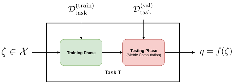
Consider the mapping between hyperparameters and the metric that is being optimised. Given a specific configuration of hyperparameters, say $\zeta \in \mathcal{X}$ where $\mathcal{X}$ denotes the space of hyperparameters, we train the model and monitor validation-set performance via some metric, say $\eta$, then we can represent this mapping to be a function $f$ s.t. $f(\zeta) = \eta$. Our goal is to optimise this function over the space of all hyperparameters. Note that, often, it is hard to run a grid-search over all sets of hyperparameters because deep models are expensive to train. Thus, we can assume that we have information about this function $f$ only on a small set of points, $\zeta_{1}, \zeta_{2}, .., \zeta_{N}$. This poses itself as an optimisation problem with knowledge of the to-be-optimised function on a small number of points. For this reason, this functional mapping is called as the black-box function. Formally, assuming we are trying to maximize the metric, the optimisation problem we are trying to solve is:
\[\zeta_* = \arg\max_{\zeta \in \mathcal{X}} f(\zeta) \ \ \ \text{s.t.} \ f(z_{n}) = \eta_{n}, \ \forall n \in \{1, 2, .., N\}\]This optimization is at two levels: Firstly, we are trying to achieve a reasonable estimate of the black-box function $f$, and secondly, we are trying to reach to the optima of this blackbox function.


Bayesian Optimisation for Hyperparameter Tuning
We assume that we have a set $\mathcal{D} := (\zeta_{n}, \eta_{n})_{n=1}^{N}$ of observations. We assume a likelihood model with noise as
\[\eta_{n} \approx f(\zeta_{n}) \leftrightarrow \eta_n = f(\zeta_n) + \epsilon\]for the limited amount of evaluations of $f$ we have. We also assume a prior on the behavior of $f$. As usual, we infer a posterior over $f$ and use this posterior information to find points in the search space $\mathcal{X}$ that can help us reach the optima. In order to find new points in $\mathcal{X}$, we define an aquisition function
\[a : \mathcal{X} \rightarrow \mathbb{R}\]This aquisition function controls the \textit{exploitation-exploration} trade-off. By exploitation, we mean that select new points from the region where we suspect the optima exists. For instance, if we are minimizing the black box function, then we will choose points on which the values of $f$ would be lower. By exploration, we set out finding points in the search space where we have very little observations about the behavior of $f$. Once we have found a new point, we evaluate $f$ on it and add it to the dataset $\mathcal{D}$ and update the posteriors and continue the procedure until some convergence criterion. Now, we will give a detailed account of using Bayesian optimization for choosing near-optimal hyperparameters. Let us say we have a machine learning task $T$ at hand. We have data $\mathcal{D}_{\text{task}} $ that we can use to train and test the model for task $T$. Let’s assume some split of the dataset.
\[\mathcal{D}_{\text{task}} = \mathcal{D}^{(\text{train})}_{\text{task}} \cup \mathcal{D}^{(\text{val})}_{\text{task}} \cup \mathcal{D}^{(\text{test})}_{\text{task}}\]Let’s say the model for $T$ has hyperparameters $\zeta \in \mathcal{X}$ and the metric w.r.t which they are to be optimized be $\eta \in \mathbb{R}$. Assume $\zeta$ is $K$ dimensional with its components being continuous, categorical or ordinal. The hyperparameters are related to the concerned metric by the black-box function.
\[f: \mathcal{X} \rightarrow \mathbb{R}; \ \ f(\zeta) = \eta\]
Considering the task T as an oracle which on input $\zeta$ outputs a metric value $\eta$, we now articulate the Bayesian optimization routine. Let’s say we have a surrogate model which models $f$ and we assume some prior $p(f)$ on $f$. Let the hyperparameters if the surrogate model and the prior together be denoted by $\Theta$.
- Initialization: Construct initial dataset with mapping of $\zeta_k$ to $\eta_k$ for $N$ such points.
- Repeat until convergence: (Can monitor some meta-metric to check convergence)
- Compute the posterior predictive distribution mean and variance: $ mean(\zeta | D_{surrogate}, \Theta) $, $ var(\zeta | D_{\text{surrogate}}, \Theta), \ \forall \zeta \in \mathcal{X} $.
- Use the predictive mean and variance to compute the expected improvement $ \alpha_{EI}(\zeta), \forall \ \zeta \in \mathcal{X}$
- Choose a new point $\zeta_{new}$ based on maximum expected improvement. $\zeta_{new} = \arg\max_{\zeta \in \mathcal{X}} \alpha_{\text{EI}}(\zeta)$
- Pass $\zeta_{new}$ to the task T in order to compute $\eta_{new} = f(\zeta_{new})$.
- Add $(\zeta_{new}, \eta_{new})$ to $D_{\text{surrogate}}$. Update the posterior and continue.
The properties we can extract from a Bayesian optimization model depend upon the choice of surrogate model we use to approximate the black-box function and the kind of acquisition function we use in the routine.
Choice of surrogate model
Typically, the most popular choice for surrogate model has been Gaussian Processes. A key limitation of GP based surrogate model is that its computational complexity scales cubicly in the number of examples. This is due to the matrix inversion of an N × N matrix during the posterior computation in GPs. This restricts the usability of GPs in a setting where large number of black-box function evaluations are necessary for reliable estimates. As a seminal work in this area, Snoek et al [9] introduce usage of Bayesian neural networks as a replacement to GPs to model the black-box function. They show impressive results on variety of vision and natural language tasks with the black box function being modelled by a fully-connected network with Bayesian linear regression on the last layer.
Choice of acquisition function
The choice of acquisition function to choose a new point in a sequential optimizer gives over the exploration-exploitation trade-off. Expected improvement [5] is one of the most popularly used method for choosing a new point in the optimization space in a sequential optimization based model.
\[\alpha_{EI}(\textbf{x}| \mathcal{D}, \theta) = \sigma(\textbf{x} | \mathcal{D}, \theta)\left( \gamma(\textbf{x})\Phi(\textbf{x}) + \mathcal{N}(\gamma(\textbf{x}) | 0, 1) \right)\] \[\text{where} \ \ \gamma(\textbf{x}) := \frac{f(\textbf{x}_{best}) - \mu(\textbf{x} | \mathcal{D}, \theta)}{\sigma(\textbf{x} | \mathcal{D}, \theta)}\]It is noted in the literature that the EI criterion tends to be too greedy (exploitative) in nature. There is a recent work [8] that improves the criterion in the direction of making it more exploratory. Even in our preliminary experiments, we observed that the vanilla EI criterion tends to exaggerate the exploitative behavior.
Experiments and Results
We borrowed a simple implementation of Bayesian neural network from pybnn as our base model on which we built the Bayesian
optimization routine. Our goal is to check Snoek et al [9] work on scalable Bayesian optimisation on a bunch of simple tasks:
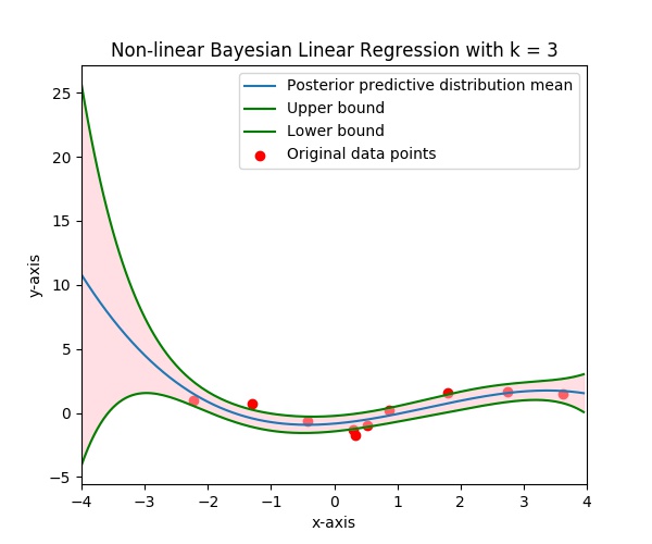
- Task 1: Bayesian Linear Regression on a toy-dataset We consider a toy-dataset and the task is to learn a Bayesian linear regressor on a hard-coded kernel on the one-dimensional dataset. The dataset consists of 10 data points and was provided as a part of assignment 1 of the course. Please refer to assignment 1 for more details about the dataset and the task. For the purpose of this project, we consider estimation of the following hyperparameters: $K$: kernel dimension, $\lambda$: linear regression regularization hyperparameter and $\beta$: noise precision. We consider a fixed range of values for each of the parameters and discretize the space. The optimization of aquisition function operates in this discretized space. We obtained K = 3, β = 4.0, λ = 1.0 as the optimal hyperparameter configuration. This was in accordance with our Assignment 1 results. The visualization is shown in the following figure.


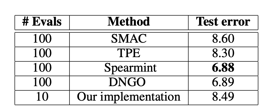
- Task 2: Logisitc Regression on MNIST dataset In order to show the efficacy of the framework on a real-world dataset, we consider the task of logisitc regression on MNIST image dataset. This is one of the simplest benchmark tasks considered in the literature of hyperparameter optimization [2]. We consider a split of 50k/10k/10k for train/validation/test. For simplicity, we only consider two hyperparameters, $C$: regularization hyperparameter, $l$: intercept-scaling parameter of the \texttt{liblinear} package. We use only these two as against the four used in relevant literature because these are readily available with the \texttt{scikit-learn} logisitic regression package. However, our code is flexible enough to incorporate other hyperparameters. We obtained {C, l} = {3.775, 1.625} as the optimal setting on which we obtained 91.51% accuracy on the test set. The comparison with relevant literature is shown in the table above.
For more details and other visualizations, please refer to our project report.